Economic Efficiency of Cap-and-Trade Systems in Carbon Emissions Reduction

Environmental Economics

Do carbon-pricing schemes cut emissions without holding back growth? I merged three global datasets in Python and tested how emissions move with GDP, population and the share of emissions covered by carbon pricing.

Context Economics Seminar, Nagoya University

Tools Python (pandas, statsmodels)

Data Our World in Data, World Bank

Sample 5,643 country-years, 1989–2021

0.977 R² of the OLS model on total CO₂

5,643 Country-year observations after cleaning and merging

0.976 Correlation between population and total CO₂

0.039 p-value on carbon-pricing coverage, which has a negative coefficient

Question

Market-based climate policy is widely adopted. Does it actually work at the macro level?

Cap-and-trade systems (ETS) set a ceiling on emissions and let firms trade permits, so the cut happens where it is cheapest. Growing GDP and population push energy demand and emissions up, so the real test is whether coverage still matters after those scale effects are accounted for.

The literature points in that direction. Zhou et al. (2021) compared cap-and-trade with carbon taxes in a CGE model and found that both affect GDP, but cap-and-trade has the smaller impact. Zhang et al. (2024) reviewed implementation at national, industry and enterprise level and its role in sustainability.

Data

Three public datasets were reformed and merged on country and year into one panel of 5,643 observations:

Carbon pricing coverage, from Our World in Data (2024). It covers the share of emissions under an ETS, under a carbon tax and in total. Over time, policymakers shift toward market-based mechanisms.
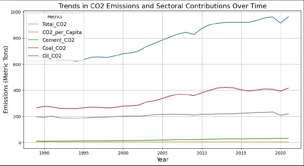
CO₂ emissions, from Our World in Data (2024). It has total, per-capita and sector series (coal, oil, cement). Per-capita emissions stay roughly flat, which hints at efficiency gains.
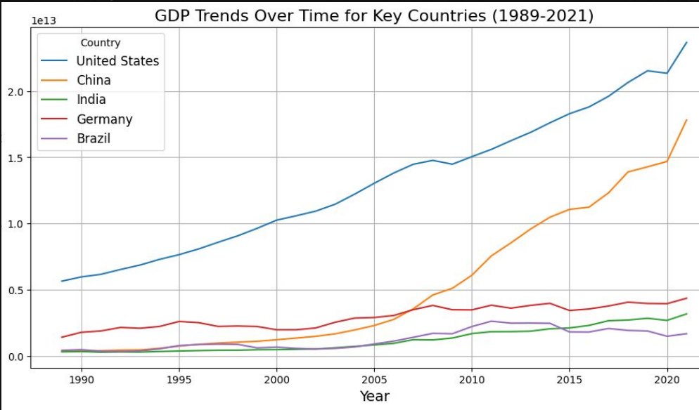
GDP, from the World Bank (2024). It has annual GDP for every country.

Line chart of total, coal, oil, cement and per-capita CO2 emissions from 1989 to 2021 — Total CO₂ climbs steadily while per-capita emissions stay flat. Coal is the largest sector.

Line chart of GDP for the United States, China, India, Germany and Brazil from 1989 to 2021 — GDP for five key economies, a sample of the full country dataset.

Method

Clean and mergeHarmonise country codes and years across the three sources and keep only the country-years present in all of them.
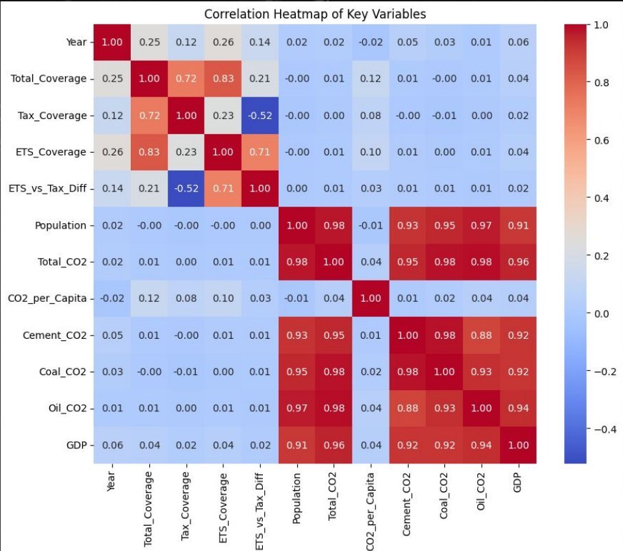
Correlation analysisBuild a full correlation matrix across coverage, emissions, population and GDP to map the relationships before modelling.
OLS regressionRegress total CO₂ on GDP, population and total carbon-pricing coverage with statsmodels.
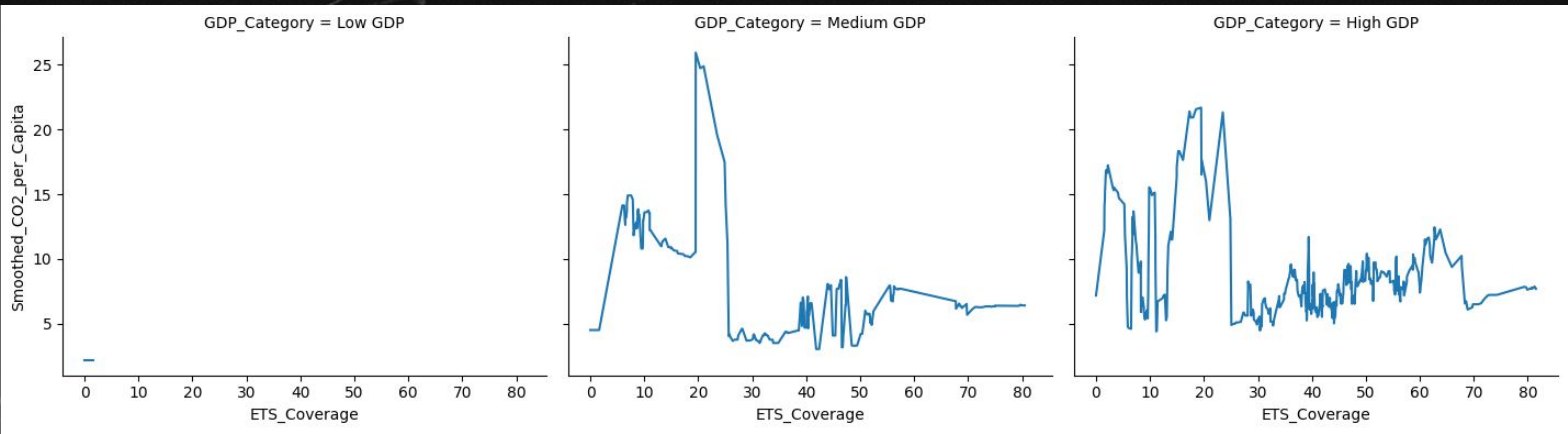
Visualise by income groupSplit countries into low, medium and high GDP groups and plot smoothed per-capita CO₂ against ETS coverage.

Results

Holding GDP and population fixed, each extra percentage point of carbon-pricing coverage is associated with about 0.57 lower total CO₂ (p = 0.039).

OLS regression · dependent variable: Total CO₂ · n = 5,643
Variable	Coef.	Std. err.	t	p	95% CI
Constant	−3.0266	5.114	−0.592	0.554	[−13.051, 6.998]
GDP	2.037e−10	2.59e−12	78.714	0.000	[1.99e−10, 2.09e−10]
Population	2.81e−06	2.27e−08	123.899	0.000	[2.77e−06, 2.85e−06]
Total coverage	−0.5674	0.275	−2.066	0.039	[−1.106, −0.029]

R² 0.977 · Adj. R² 0.977 · F 8.002e+04 · Durbin–Watson 0.130 · Cond. no. 4.93e+12

What drives emissions

Scale effects dominate. Population (r = 0.976) and GDP (r = 0.956) move almost one for one with total CO₂.
Growth is not carbon intensity. GDP barely correlates with per-capita emissions (r = 0.042).
ETS drives coverage. ETS coverage correlates 0.831 with total coverage, so trading schemes are how most emissions get priced.

Correlation heatmap of coverage, emissions, population and GDP variables — Correlation heatmap of the merged dataset. The red block on the lower right is the population, GDP and emissions cluster.

Three panels of smoothed CO2 per capita against ETS coverage for low, medium and high GDP countries — Smoothed per-capita CO₂ against ETS coverage by income group. In medium- and high-GDP countries, emissions per person fall sharply once coverage passes about 25%.

Limitations

The model explains almost all the variance, but that is mostly the scale variables doing the work. Read it with care:

Multicollinearity. GDP, population and emissions are highly correlated (condition number 4.93e+12), which makes individual coefficient estimates less reliable.
Serial correlation. A Durbin–Watson statistic of 0.130 means residuals are strongly autocorrelated across years, as expected in pooled country-year data.

Next iteration

Country and year fixed effects to strip out level differences and global shocks.
Standard errors clustered by country.
Log-transformed GDP, population and emissions to read coefficients as elasticities.

Analysis of The Minimum Wage & The Gig Economy of Indonesia Next case study